Efficiently counting complex multilayer temporal motifs in large-scale networks

Abstract

This paper proposes novel algorithms for efficiently counting complex network motifs in dynamic networks that are changing over time. Network motifs are small characteristic configurations of a few nodes and edges, and have repeatedly been shown to provide insightful information for understanding the meso-level structure of a network. Here, we deal with counting more complex temporal motifs in large-scale networks that may consist of millions of nodes and edges. The first contribution is an efficient approach to count temporal motifs in multilayer networks and networks with partial timing, two prevalent aspects of many real-world complex networks. We analyze the complexity of these algorithms and empirically validate their performance on a number of real-world user communication networks extracted from online knowledge exchange platforms. Among other things, we find that the multilayer aspects provide significant insights in how complex user interaction patterns differ substantially between online platforms. The second contribution is an analysis of the viability of motif counting algorithms for motifs that are larger than the triad motifs studied in previous work. We provide a novel categorization of motifs of size four, and determine how and at what computational cost these motifs can still be counted efficiently. In doing so, we delineate the “computational frontier” of temporal motif counting algorithms.

Introduction

The field of network science [1], also referred to as (social) network analysis [2], aims to understand complex systems by studying the interactions between entities within such a system as a network. Examples include (online) social networks, communication networks, collaboration networks, and economic networks.

Over the past years, at least four developments have affected the field. First, there is an ever increasing desire to understand and learn from network dynamics, i.e., the temporal evolution of networks [3, 4]. Second, different types of interactions may be observed between nodes in the network, forming the so-called multilayer networks [5] (sometimes referred to as multiplex networks, see [6] for a discussion on terminology). It has repeatedly been shown that taking multiple types of interaction into account can result in novel insights that would not be discovered when layers were aggregated or analyzed individually. Third, with the wide availability of data from the Internet, social media websites, and online platforms, there is more and more need to analyze large-scale networks with millions of nodes and links, requiring highly efficient algorithms. Fourth, many studies in network science limit themselves to attempting to explain macro-level properties of the network as a whole (e.g., degree distributions), using microlevel properties of the nodes (e.g., node degrees). However, in recent years, it has been shown that there are also noteworthy patterns at the meso-level of a network. One example of such a meso-level pattern is a network motif: a small configuration of a few nodes and edges that occurs throughout the network at a high rate [7, 8]. These motifs can reconfirm the existing hypotheses about certain interaction patterns, but they can also provide new insight into previously unknown meso-level patterns and underlying behavior in the network [9,10,11,12]. In this paper, we propose an approach for counting these network motifs. Crucially, we do so in networks that (a) have temporal information, (b) consist of multiple layers, and (c) potentially contain millions of nodes and links.

Network motifs provide insights that go beyond studying either individual nodes or the network as a whole, allowing the role of groups of nodes in particular configurations to be studied. In biological networks, the regulating function of feed-forward loop motifs has frequently been identified [13]. In economic networks, motifs of corporate interlinkage were able to highlight particular corporate structures such as crossholdings [11], as well as unveil the influence of the financial sector in creating complex corporate structures [14]. And in user communication networks, specific network motifs revealed, for example, blocking behavior in online conversations [15]. Given the importance of motifs in understanding the structure of networked systems, identifying motifs and understanding their implications are of crucial importance to network science.

Research on methods and algorithms for the detection of motifs dates back to early work on the problem of mining frequent subgraphs [16]. We will henceforth refer to the task performed by these subgraph enumeration methods as motif enumeration. The advantage of algorithms for motif enumeration is that they iterate over all possible subgraphs of a given size, allowing the actual subgraphs themselves to be identified in the network, and their composition to be inspected afterwards. The clear drawback of motif enumeration is the large amount of memory required to store the obtained motifs, as well as the running time, which is typically dependent on the size of the network and grows exponentially with the size of the subgraph. Although multilayer motif enumeration algorithms have been explored [11, 17], even for patterns of a few nodes and edges, these algorithms quickly become too computationally intensive. This limits the applicability of these approaches for finding larger patterns, or for analyzing larger networks.

As an alternative to enumeration, motif sampling techniques have been introduced [18, 19]. They are extremely useful if the goal is to unveil only the most frequently occurring motifs. However, sampling methods suffer from an inherent uncertainty in their estimation. Although work on motif sampling when the structure of the network is scale-free and thus nonrandom has been done [20], the simultaneous presence of a multilayer structure makes it difficult if not impossible to derive sufficiently reliable analytical bounds on the errors of motif sampling algorithms. Practically, this means that in the multilayer setting, it is nontrivial to derive a good sampling rate, such that all motifs are discovered. Especially, if the motif counts are skewed, infrequent motifs may be overlooked. This disqualifies the use of sampling for our particular research goal: exactly counting how often all possible multilayer motifs occur in a given network.

Thus, to counter the limitations of motif enumeration and sampling, this paper builds upon recent algorithmic developments made in motif counting [7, 15, 21]. The advantage of motif counting over motif enumeration is that motif counting algorithms do not require the enormous amount of memory needed by motif enumeration to store all isomorphic subgraphs. In addition, it was shown that for motifs of size 2 and 3, time-efficient algorithms that can count motifs in networks with millions of nodes and edges in a matter of minutes can be utilized [7]. An obvious downside of motif counting is that it is no longer possible to track precisely where in the network, the motifs occur, or to determine precisely which nodes are involved in these motifs. However, it should be noted that if one is interested in only a few frequent motifs, and not all motifs, one could, after counting, simply only enumerate these few motifs, which is still far more efficient than enumerating all motifs.

Thus far, we have defined motifs (sometimes also called graphlets) as little subgraphs that frequently occur in the network. In other texts, motifs are specifically defined as subgraphs that occur more frequently than a certain threshold frequency, possibly determined based on motif frequencies in a null model. This final step, in which what is called motif significance is determined, is beyond the scope of this paper, as our focus is on counting algorithms. However, it should be noted that the trivial post-processing step for determining motif significance can easily be added, for example as described in  [11, 19].

In this work, we consider the task of counting multilayer temporal network motifs in six different temporal networks that all model communication between human users. For each link between users, we know the timestamp at which the communication took place. Examples include user communication on a social network and a network of e-mail communication between employees of a large organization. We also analyze four datasets from the so-called online expert knowledge exchange websites, where users can communicate and discuss about questions from a particular domain. The considered datasets each contain elements that one encounters when studying real-world multilayer network datasets: some of the layers of the multilayer network may be undirected rather than directed, and some layers may be partially timed or have no temporal information at all. We set out to investigate what patterns of communication, i.e., which temporal motifs, occur in these datasets, and how these motifs differ between the various networks.

Three challenges arise as a result of the research agenda set out above. First of all, existing temporal motif counting algorithms work on one-layer networks rather than multilayer networks. Second, existing efficient implementations of algorithms for motif counting do not yet incorporate partial timing, which is frequently encountered in real-world network data. Third and last, it is unclear to what extent motifs consisting of more than 3 nodes and edges can efficiently be counted using the motif counting algorithms proposed in [15]. In general, it is unknown what the possibilities and limitations of these approaches are in understanding more complex and larger patterns of interaction in temporal networks.

The main contribution of this paper is twofold. We start by introducing a solution to the first two problems above, proposing a multilayer temporal motif counting algorithm that is able to efficiently deal with partial timing. Here, we build on previous work by Paranjape et al. [15], extending the approach presented in [21]. Using experiments on various large-scale datasets, we analyze the performance of this multilayer algorithm in relation to the existing layer-agnostic motif counting algorithm. Then, using the so-called motif footprints, we analyze the obtained motifs, allowing us to understand the differences in communication patterns between users in the various online platforms represented by the data. An open source implementation of our algorithm is made available, ensuring that the approach can easily be reused in future studies.

The second contribution is theoretical and entails an in-depth analysis of larger motifs, in particular those of size 4. We introduce a categorization of size motifs, and outline precisely for which categories of larger motifs which we can still employ motif counting algorithms efficiently. As such, we explore and delineate what one could call the “computational frontier” of efficient motif counting algorithms in large-scale complex networks.

The remainder of the paper is organized as follows. First, relevant related and previous work is presented in the "Related work" section. Then, the "Multilayer temporal motifs" section provides the necessary background and definitions related to our object of study: multilayer temporal motifs. Next, the proposed algorithms to count these motifs are outlined in the "Multilayer counting algorithms" section. Then, in the "Counting larger motifs" section, the analysis of how these types of algorithms may scale to larger motifs is presented. The "Datasets" section describes the real-world network datasets used in the "Experiments" section to perform experiments. Finally, the "Conclusion and future work" section summarizes our results and contributions and provides suggestions for future work.

Related work

In this section, we discuss work related to the various subproblems of counting multilayer temporal motifs, in particular distinguishing between methods for motif enumeration, motif counting, multilayer networks, and temporal networks.

One subproblem is counting or enumerating of static motifs, ignoring the network dynamics. Three categories of static motif enumeration exist: all-motif enumeration, single-motif enumeration, and motif-set enumeration. The first category, all-motif enumeration, comes closest to pure counting, as it enumerates all motifs of size k in the network. A well-known algorithm to perform all-motif enumeration is ESU, aka FANMOD [19, 22, 23]. It starts from each node and enumerates all motifs of size k that contain only that node and higher labeled vertices. This algorithm allows parallel execution from each node. Due to the skewed degree distribution in real-world networks, i.e., few nodes have a relatively high degree, some nodes will be involved in a relatively high number of motifs which leads to unbalanced parallel tasks. Shahrivari and Jalili [24] introduced an improvement on ESU named PSE. Instead of starting the enumeration from each node, PSE starts from each edge. In addition, the authors introduced the Subenum algorithm which includes two-phase subgraph isomorphism detection and ordered labellling. Experimentally, Subenum was shown to reach near-linear speed-up when adding additional threads of execution and clearly outperformed previous all-motif enumeration algorithms.

Single-motif and motif-set enumeration are, for example, useful for enumerating motifs that are found to be interesting based on pure counting results. Grochow et al. [25] introduced a single-motif counting algorithm. This algorithm was one of the first to map the motif onto the network instead of enumerating all subgraphs and testing for subgraph isomorphism. Furthermore, it takes advantage of subgraph symmetries to avoid spending time finding a motif more than once, and introduces subgraph hashing which significantly reduces isomorphism tests needed. The motif-set enumeration algorithm g-tries, introduced by Ribeiro and Silva [26], utilizes the fact that motifs can share a common subgraph to create the so-called g-tries: trees where each level adds a node to the motifs which it represents. These g-tries are used to map motifs onto the network. Like the single-motif algorithm by Grochow et al. [25], it also uses symmetry breaking. Experimentally, the authors showed that g-tries outperforms the algorithm by Grochow et al. when querying the same set of motifs.

For static motif counting, it is often most efficient to consider the structure of the motifs that you wish to count. For example, Marcus and Shavitt [27] presented efficient counting algorithms for several 4-node motifs. The authors did so by providing a separate algorithm for several types of 4-node motifs: the tailed triangles, four-nodal cliques, four-nodal cycles, and four-nodal paths and claws. As expected from pure counting algorithms, the authors proved experimentally that their counting algorithms outperformed the all-motif enumeration algorithm FANMOD (ESU).

Gonen and Shavitt [28] introduced local motif counting algorithms to count the number of motifs which a single node is involved in, as well as an approximation algorithm for the number of motifs for the entire network. They introduced algorithms for counting k-length cycles (with a chord), ($k-1$)-length paths, tailed triangles, and 4-cliques.

For multilayer motifs, we need to look at more recent work. In February 2017, Kivela and Porter [29] extended the graph isomorphisms to multilayer networks. Furthermore, they extended it to temporal networks by representing them as multilayer networks. This can be done by considering temporal networks as time sequence graphs. These extensions provided a foundation for further research of multilayer networks, such as motif analysis. In March 2017, Battison et al. [17] examined how many subgraphs exist for motifs with a small number of nodes and applied multilayer motif analysis on a brain network. However, they did not describe how they actually counted/discovered the multilayer motifs. In October 2017, Enright and Meeks [30] investigated the parameterized complexity of counting small subgraphs in multilayer networks. The authors found that if all but one of the layers are drawn from classes of bounded vertex cover number or all of the layers have almost bounded degree, then the problem is FPT (fixed-parameter tractable); otherwise, it is W[1]-hard. In November 2017, Takes et al. [11] performed multiplex motif enumeration on a corporate network. The authors proposed a multiplex adaptation of Subenum, where a multiplex graph is converted into a directed labeled graph. An edge label then encodes which edge types are and are not present between the two nodes that it connects. Furthermore, the authors build on the stub-matching model [31] for the null model to preserve interlayer assortativity [5].

The temporal motif problem has developed over the years to more accurately capture the timing information. In 2009, Braha and Bar-Yam [3] took snapshots of the network, where each snapshot covered a single day. However, the snapshots themselves lose the information regarding the order of events. In 2010, Zhao et al. [32] considered two events (edges) linked if they share a node and succeed one another within a time limit $\varDelta t$. However, this enforces only local time adjacency. Kovanen et al. [33], in 2011, called such events $\varDelta t$-adjacent and considered two events $\varDelta t$-connected if there is a sequence of $\varDelta t$-adjacent events joining them. A temporal motif is then defined as a set of events that are all $\varDelta t$-connected. Finally, in February 2017, Paranjape et al. [15] count temporal motifs where every pair of edges is at most $\delta$ time apart, thus fully utilizing the timing information. We build upon these techniques, which we henceforth refer to as the delta-time-window approach, adding both partial timing and functionality to handle multiple network layers.

Multilayer temporal motifs

In this section, we provide necessary definitions and introduce notation for the algorithms described in the remainder of this paper. We follow the notation and definitions introduced in [15] and build upon the definitions in [21].

We consider the basic building block of a network structure to be an edge: a (directed) link between an ordered pair of nodes. It can be defined as a tuple (u, v) with u denoting the source node and v the target node. Given a node set V of size $n = |V|$, a static graph $G = (V, E)$ is defined by a set E containing edges $(u_i,v_i)$, for $i=1,2,\ldots ,m$, with $u_i,v_i \in V$. For temporal edges, we add a timestamp t, and for layered edges we add a layer number l. Thus, in a multilayer temporal graph H, an edge is defined as $(u_i,v_i,t_i,l_i)$, where $t_i \in \{-1\}\cup \mathbb {R}^{+}$ and $l_i \in \{1,\dots ,\varLambda \}$, with $\varLambda$ the number of layers. A timestamp of $-1$ indicates that there is no known timestamp for that edge (in case of partial timing). Note that this introduces simultaneous edges, i.e., edges with the same timestamp. The underlying static graph of a multilayer temporal graph is the graph formed by ignoring all timestamps, layers, and duplicate edges. For the algorithms in this paper, we assume edges to always be directed. However, results for undirected edges can be obtained through post-processing. This leads us to the following definition.

Definition

A r-node, s-edge, $\delta$-temporal, $\lambda$-layer motif is a sequence of s edges, $M = ((u_1,v_1,t_1,l_1), (u_2,v_2,t_2,l_2), \dots , (u_s,v_s,t_s,l_s))$ that are time-ordered within a $\delta$ duration, i.e., $t_1< t_2< \cdots < t_s$ and $t_s - t_1 \le \delta$, and range over at most $\lambda$ different layers, such that the underlying static graph is connected and has r nodes.

Note that multiple edges between the same pair of nodes are possible and individually counted and that timestamps induce an ordering on the edges. Furthermore, this definition allows $\lambda$ different layers in the motif M, but also allows fewer layers. For example, Fig. 1b (e.g., $M_{1,3,3}$) shows a 3-node, 3-edge, $\delta$-temporal, 3-layer motif including just 2 layers, given a suitable $\delta$. We say that a motif $M = ((u_1,v_1,t_1,l_1),\dots , (u_s,v_s,t_s,l_s))$ occurs in a multilayer temporal graph H when there is a time-ordered sequence $S = ((w_1,x_1,t'_1,l'_1), \dots ,(w_s,x_s,t'_s,l'_s))$ of s unique edges in H, such that

• 1. there exists a bijection f, such that $f(w_i) = u_i$ and $f(x_i) = v_i\ (i=1,\dots ,s)$,

• 2. the edges all occur within $\delta$ time, i.e., $t'_s - t'_1 \le \delta$, and

• 3. there exists a bijection g on the layers, such that $g(l'_i) = l_i\ (i=1,\dots ,s)$, which holds for all motifs within a single search.

Each such sequence of edges is called an instance of the motif M, and the goal of this paper is to count the number of such instances. The main problem, for which algorithms are proposed in the "Multilayer counting algorithms" section, is as follows:

Given set values for $r,\ s,\ \delta$ and $\lambda$ and a multilayer temporal graph H, compute the number of occurrences of each motif.

Fig. 1

Overview of different motif types. a All 2,3-node, 3-edge δ-temporal motifs (Figure from [15]. The edge numbers indicate their temporal order. b All 3-layer variants of M_1,3

The fast algorithms presented in [15] focus on 2,3-node (i.e., 2 or 3 nodes), 3-edge $\delta$-temporal motifs, providing the overview of all such motifs in Fig. 1a. In the "Counting larger motifs" section, we investigate whether these methods can be extended to count 4-node, 4-edge motifs. Returning to the multilayer aspect, crucially, we note that altering an edge’s layer does not affect the temporal order or edge configuration. Therefore, every $\delta$-temporal $\lambda$-layer motif can be associated with a single $\delta$-temporal motif. Figure 1b shows all 3-node, 3-edge, $\delta$-temporal, 3-layer motifs, given a single $\delta$-temporal motif $M_{1,3}$ from Fig. 1a. The number of associated $\delta$-temporal $\lambda$-layer motifs for a single $\delta$-temporal motif depends on the number of possible layer permutations. Therefore, for each s-edge, $\delta$-temporal motif, there exist $\lambda ^s$ $\delta$-temporal, $\lambda$-layer motifs. Thus, there are $3^3 \times 36 = 972$ 2,3-node, 3-edge, $\delta$-temporal, 3-layer motifs.

To reference one $\delta$-temporal $\lambda$-layer motif, we add a layer-specific index into the possible permutations of Fig. 1a. For 3-layer networks, the $3^3 = 27$ layer permutations are shown in Fig. 1b. Note that in this figure, motifs 1, 2, 4, 5, 10, 11, 13, and 14 are in total $2^3 = 8$ permutations of 2-layer motifs.

Multilayer counting algorithms

In this section, we will first present the multilayer algorithms, which are extended versions of the algorithms proposed as part of the delta-time-window approach discussed in [15], now incorporating both the multilayer aspect as well as partial timing. The multilayer general algorithm is discussed in the "General motif counting" section, and multilayer 3-node star and triangle motif counting algorithms are presented in the "Star motif counting" section and the "Triangle motif counting" section.

General motif counting

The general algorithm for counting the number of instances of (multilayer) temporal motifs consists of a 3-step procedure. First, all instances $U'$ of the static motif U, underlying M, in the static graph G, underlying the multilayer temporal graph H, are identified. This can be accomplished with known algorithms for enumerating static motifs. Second, for each motif instance $U'$, all temporal edges between pairs of nodes forming an edge in $U'$ are gathered into an ordered sequence $S'$. We extend this step, by filtering these temporal edges, such that the layers from the edges match those in U. We denote the resulting sequence of edges by $S''$, which then consists of only those edges required to count the instances of our multilayer temporal motif U. Finally, the number of subsequences of edges in $S''$ occurring within $\delta$ time units that correspond to instances of M are counted. Algorithm 1 describes the algorithm used to identify and count these subsequences. Note that the second and third steps of this algorithm can be done in parallel for each static motif $U'$ found in the first step.

When simultaneous edges occur, the order of the edges is determined not by their timestamp but their order in the sequence $S''$. In the case of partial timing with a layer consisting of only untimed edges, the resulting motif counts can easily be post-processed to obtain the same result for every ordering. However, if a layer itself is partially timed, the order of simultaneous edges has an impact on the resulting motif counts. Therefore, on an implementation level, to ensure consistent output, we have enforced this to be the order in which the edges appear in the input file.

Partial timing With respect to the original algorithm in [15], the highlighted code in Algorithm 1 denotes the changes for partial timing. In lines 2–3, we loop over all untimed edges and increase the relevant counters and subsequently never decrement any counters given these edges. In other words, untimed edges are never forgotten, acknowledging that they could have formed at any given time and should be considered part of every delta-timeframe. However, this approach does mean that the untimed edges are always considered to be the first in the order of events. To ensure that we can decrement the counters correctly in the main for loop (lines 4–7), we keep track of these untimed edges in separate counters “pcounts[.]”. The additional updates, incrementing and decrementing, of the counters, based on these “pcounts” counters, are done in lines 17 and 14, respectively. These updates take into account that untimed edges counted in “pcounts” are always first, which is why a prefix is used for decrementing instead of a suffix. On an implementation level, the additional for loop in lines 13–14 can easily be merged with the preceding for loop. Thus, we only add a small number of operations per edge which should not significantly impact the algorithm’s time complexity. Furthermore, any untimed edges will now only require a call to IncrementCounts, reducing the average number of operations per edge the more untimed edges there are.

Multilayer aspect The addition of multiple layers is realized by adding a parameter l to each edge-related parameter. For example, in line 10, we only need to change the variable e to include the associated layer (e, l). These changes only really impact the number of possible keys for the array “counts[.]”.

As the overall approach of our multilayer algorithm does not differ from that of the original one-layer algorithm, the same arguments for efficiency still apply. This means that it will perform with linear complexity for 2-node motifs, but its use for 3-node and larger motifs would be inefficient. Therefore, we also extended the faster 3-node algorithms to the multilayer perspective described below.

Star motif counting

Star motifs are motifs that consist of a center node u and edges to $r-1$ neighbors, with no edges connecting these neighbors. Example star motifs are $M_{1,1}$, $M_{1,5}$, and $M_{5,5}$ in Fig. 1a. We define each edge in a star motif by its neighbor node (nbr), its direction towards or away from u (dir), its timestamp (t), and its layer (l). For the multilayer triangle and star algorithms, we will look specifically at 3-node 3-edge $\lambda$-layer star motifs. The static motifs underlying these star motifs can be divided into three classes: pre, post, and mid, as depicted in Fig. 2. While processing the time-ordered sequence of edges, we consider the current edge being processed as the singular edge in the motifs, i.e., edge 3 for pre. Algorithm 2 provides the algorithmic framework for the triangle and star counting algorithms, with full multilayer implementations of Push(), Pop(), and ProcessCurrent() in Algorithm 3.

Fig. 2

(figure from [15])

The pre, post, and mid classes of temporal star motifs

Partial timing The highlighted code indicates the changes required for handling partially timed networks. Just like for the general algorithm, we first require the untimed edges to be preprocessed (lines 4–9). For each counter, we add a p-preceded counter to count the untimed edges. Furthermore, the procedures are updated with a type parameter which determines which operations are and are not performed. When they are called with type set as indicated in Algorithm 2, we count considering partially timed motifs. However, if they were all set to 0, the algorithm would function no different than the original one-layer algorithm.

During the preprocessing in lines 4–9, the fully untimed motifs are counted. For partially timed pre motifs, we account for untimed edges in lines 21, 27, and 31, in the same manner as we did for the general algorithm earlier. To count partially timed mid motifs, we must distinguish between two cases. First, we must consider the single edge, edge 2, to be timed. In this case, we require an additional type of mid motif counter ($ppre\_mid$), which is used to count the number of combinations of edges 1 and 3 of the mid type motif found. We require this additional counter, because unlike all other cases this counter counts both an untimed and a timed edge. It is updated in lines 22 and 30 and used to update the motif counter in line 33. The second case considers the single edge to be untimed. In this case, only the third edge would be a timed edge and all these edges are added to the $ppost\_nodes$ counter in lines 4–5. Subsequently lines 8, 33, and 34 ensure these partially timed mid motifs which are counted during the preprocessing stage. Similarly, all partially timed post motifs are counted by lines 4–5, 8, and 32.

Multilayer aspect We can see that adding layers does not change the main method of operation, but only requires us to add a layer index for every direction index to each counter. Therefore, we update the original counter definitions to the following:

• pre_nodes[dir, $v_i$, l] counts the number of times node $v_i$ has appeared in an edge alongside u with direction dir and layer l in the timeframe [$t_j-\delta , t_j$)

• pre_sum[$dir_1$, $l_1$, $dir_2$, $l_2$] counts the number of sequentially ordered pairs of edges in [$t_j-\delta , t_j$) with the first edge having direction $dir_1$ in layer $l_1$ and the second edge direction $dir_2$ in layer $l_2$

• count_pre[$dir_1$, $l_1$, $dir_2$, $l_2$, $dir_3$, $l_3$] counts the full motifs found within $\delta$ time, with $dir_1$, $dir_2$, and $dir_3$ indicating the directions and $l_1$, $l_2$, and $l_3$ indicating the layers of the three edges, respectively

• post_nodes[dir, $v_i$, l], post_sum[$dir_1$, $l_1$, $dir_2$, $l_2$], and count_post[$dir_1$, $l_1$, $dir_2$, $l_2$, $dir_3$, $l_3$] analogous to the pre counters but for the timeframe ($t_j$,$t_j + \delta$].

• mid_sum[$dir_1$, $l_1$, $dir_2$, $l_2$] counts the number of pairs of edges where the first edge is in direction $dir_1$, with layer $l_1$, and occurred at time $t<t_j$ and the second edge is in direction $dir_2$, with layer $l_2$, and occurred at time $t'>t_j$, such that $t'-t\le \delta$

• count_mid[$dir_1$, $l_1$, $dir_2$, $l_2$, $dir_3$, $l_3$] analogous to the pre and post counters.

In the "Complexity of multilayer triangle and star algorithms" section, we will discuss how including layers does impact the space and time complexities of the algorithm.

Note that, like the original algorithm [15], our multilayer algorithm also includes instances of 2-node motifs, which we subtract from the count using the multilayer general algorithm (as this algorithm is still optimal for size 2). The full process of counting multilayer temporal star motifs is then:

• 1. for each node u in the multilayer temporal graph H, consider u as the center node and get a time-ordered list of all edges containing u;

• 2. use Algorithms 2 and 3 to count star motifs;

• 3. for each neighbor v of u, subtract the 2-node motif counts using Algorithm 1.

This procedure can be done in parallel for each node u.

Triangle motif counting

Triangle motifs are motifs where the edges form a triangle (see Fig. 1b). We define each triangle by nodes u and v and a common neighbor. Each edge in a triangle motif is defined by a neighbor node, an indicator whether it is connected to u or v (uorv), a direction, a timestamp, and a layer. The algorithmic framework, defined in Algorithm 2, used to count star motifs, can also be utilized for triangle motifs. The new implementations of Push(), Pop(), and ProcessCurrent() are described in Algorithm 4. Note that, where the process for star motifs could be parallelized for the center node, it can now for each connected node pair u, v. After all, if we consider a connected node pair u, v to be the center node, then the triangle motif has two edges to one neighbor, just like a star motif, and a self edge, which we can view as the edge to the second neighbor of a star motif.

Therefore, unlike for counting star motifs, when we count triangle motifs we do not have a single-center node and two neighbors, but two center nodes and one neighbor. This means that we must distinguish between behaviour for updating using an edge connected to u or v. Therefore, all counters are updated with an additional field (uorv) which determines if the first edge was either connected to u or v. The edge between u and v is used as the final edge to complete the triangle. To this end, these edges are only processed in ProcessCurrent() in lines 36–43. Again, the highlighted code indicates the updates for counting partially timed motifs. We can see that these changes are very similar to those for star motifs, so we will not discuss them in detail. Analogously to the one-layer algorithm, we assign each triangle to the pair of nodes with the largest edge count, so that as many triangles as possible are processed at once.

Complexity of multilayer triangle and star algorithms

Our multilayer algorithm has time complexity $O(|S''|)$, i.e., is linear in the size of the filtered sequence of edges. This is due to the fact that the mode of operation is essentially the same as the original one-layer algorithms [15] and that only the relevant layers remain in $S''$. This is different for Algorithms 2 and 3. Our multilayer star algorithm performs $O(\lambda )$ operations for both Push and Pop functions and $O(\lambda ^2)$ for ProcessCurrent, adding $O(\lambda ^2)$ operations for each edge. This also holds for partially timed networks. However, for small $\lambda$, $\lambda ^2$ is negligible with respect to time complexity, i.e., $O(\lambda ^2)$ would in practice add only a constant, and the multilayer algorithm remains linear in the size of the input sequence. Note that for a one-layer network, $O(\lambda ^2) = O(1)$. Similarly, for our multilayer triangle algorithm, we go from an original complexity of O(1) to $O(\lambda ^2)$.

Compared to the original algorithm, the sizes of the “sum” and “count” counters increase, respectively, by a factor of $\lambda ^2$ and $\lambda ^3$. With small $\lambda$ and the largest of these data structures being of size $8\lambda ^3$, the space requirements for these counters are negligible. However, the “nodes” counters require a far greater amount of space. In our multilayer algorithm, we increase the size of the “nodes” counters by a factor $\lambda$. Thus, each “nodes” counter consists of $4\lambda k$ integers, where k is the number of neighbors. In the worst case, all other nodes are neighbors and k equals $n - 1$. Therefore, the much smaller factor $\lambda$ is negligible in space complexity.

Counting larger motifs

In this section, we explore motifs with more than 3 nodes and edges. Specifically, we determine which motifs can still be counted faster than $O(m^2)$. Larger motifs are of interest, because only a small set of meaningful interaction patterns can be captured with 3 nodes. For example, in [11], several meaningful 4- and 5-node multiplex motifs were extracted from corporate networks. In biological networks, it is not uncommon for motifs to consist of a much larger number of nodes and edges. For example, in [25], in protein–protein interaction networks, meaningful motifs consisting of up to 20 nodes and 27 edges were found.

The first step in extending the algorithms introduced in [15] (and explained in a multilayer context in the "Multilayer counting algorithms" section) is to add a single node and edge. Therefore, we focus specifically on 4-node, 4-edge, $\delta$-temporal, $\lambda$-layer motifs in the "Categorization of 4-node, 4-edge motifs" section. We categorize these motifs into various types and investigate whether each of these types could be counted using a similar approach as used for 3-node, 3-edge motifs. We find that there is one particular constraining phenomenon, namely that of neighbor loops, that in some cases hinders us from handling such larger motifs efficiently, as explained in the "Neighbor loops" section. In the "Complexity of algorithms and counting approach viability for larger motifs" section, we discuss the viability of counting other size motifs using the delta-timewindow approach within $O(m^2)$ time.

Categorization of 4-node, 4-edge motifs

In this section, we take a particular interest in 4-node, 4-edge motifs. Much like for 3-node, 3-edge motifs, every 4-node, 4-edge multilayer temporal motif is directly associated with a 4-node, 4-edge temporal motif. In the previous section, we also discovered that the approach to counting temporal motifs does not change when we allow multiple layers. Since we wish to investigate if the same type of approach also works for the larger motifs, outside of data structure and algorithm descriptions, we omit layer-related aspects.

We define each 4-node, 4-edge motif to consist of two connected nodes u and v and two neighbor nodes x and y. In all following 4-node, 4-edge motif figures, the top left node is considered to be u and the bottom left node v. The 3-node, 3-edge motifs could be split into two types of motifs: star and triangle motifs. Similarly 4-node, 4-edge motifs can be split into five types of motifs:

• Square or circle motifs (sq) are motifs that form a square. Such a motif consists of the edges (u, v), (u, x), (v, y), (x, y) regardless of the direction of the edges. An example Square motif is shown in Fig. 3a.

  Fig. 3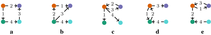

  

  Types of 4-node, 4-edge, temporal motifs. a Square, b Tailed-triangle, c Star, d Mid-Path, e Head-Path

• Tailed-Triangle motifs (tt) are motifs that form a triangle and have an additional “tail”. Such a motif consists of the edges (u, v), (u, x), (v, x), (v, y) regardless of the direction of the edges, where (v, y) is of course the tail. An example Tailed-Triangle motif is shown in Fig. 3b.

• Star motifs (st) are motifs with all edges connecting to a single node. Such a motif consists of the edges (u, v), (u, x), (u, x), (u, y) regardless of the direction of the edges. An example Star motif is shown in Fig. 3c.

• Mid-Path motifs (mp) are motifs that form a path of length three with a double edge at its center. Such a motif consists of the edges (u, v), (u, x), (u, v), (v, y) regardless of the direction of the edges. An example Mid-Path motif is shown in Fig. 3d.

• Head-Path motifs (hp) are motifs that form a path of length three with a double edge at the head of the path. Such a motif consists of the edges (u, v), (u, x), (u, x), (v, y) regardless of the direction of the edges. An example Head-Path motif is shown in Fig. 3e.

We denote each of these motifs using the index shown in parentheses (e.g., tt). Each of these types has a number of different variations, given temporal edges. Figure 4a–e provides overviews of these different variations for each respective type. For readability, the figures only show undirected variants of these motifs; the $2^4$ directed variations can trivially be derived. All other 4-node, 4-edge temporal motifs are isomorphic to one of these variations. For every type, we discuss how the concepts of the fast algorithms from the previous section can be applied. The Tailed-Triangle, Mid-Path, and Head-Path motifs will be discussed in the "Tailed-Triangle, Mid-Path, and Head-Path motifs" section, Star motifs in the "Star motifs" section, and Square motifs in the "Square motifs" section.

Fig. 4

Overview of all 4-node, 4-edge motif temporal variations per type. a Square motifs, b Tailed-triangle motifs, c Star temporal motifs, d Mid-Path motifs, e Head-Path motifs

Tailed-Triangle, Mid-Path, and Head-Path motifs

For Tailed-Triangle, Mid-Path, and Head-Path motifs, we can approach the problem in a similar way as in the "Triangle motif counting" section for triangle motifs. Each of these motifs can be defined from the perspective of a single-node pair u, v. For Tailed-Triangle motifs, we take edge u, v to be part of the triangle, with the tail connected to v. Because we require the tail to connect to the node pair u, v, we cannot assign a triangle to an arbitrary edge. After all, the edge that is not directly connected to the tail cannot be used to define u, v. Thus, we must invoke the counting algorithm for every node pair connected by an edge. This means that we would go, at least, from a complexity of $O(k\sqrt{\tau })$ to worst case O(km), with $O(\tau )$ being the complexity of the fastest available out-of-the-box triangle counting algorithm, and $k = \max _{v\in V} deg(v)$. However, every node pair can be processed in parallel and only the worst case node pairs are processed in O(k) time, provided that we maintain a time complexity for the counting algorithms linear in the size of the input edge sequence. For highly parallel execution, we would then still consider this approach efficient.

For Mid-Path and Head-Path motifs, we approach the problem from the node pair u, v that defines the middle edge of the path, because every edge in the path is connected to this node pair. Analogous to Tailed-Triangle motifs, this means that we get, at least, a worst case complexity of O(km).

By approaching these motif types in this manner, we can count motifs analogously to triangle motifs. To be able to count 4-node, 4-edge temporal motifs, we need substructures that keep count for one, two, and three edges. Because the use of a delta-time-window requires us to update counters given a single edge, all of those substructures need to be updated using the knowledge of only one edge. Herein lies the biggest obstacle in counting 4-node motifs based on a node pair u, v. After all, a single edge will only contain information for (at most) one neighbor, whilst some substructures have to be updated as if we have knowledge of both neighbors. To mitigate this problem, we avoid substructures that require direct knowledge of both neighbors. Instead, we define “all” counters, which record the sum of the counts for all neighbors, so that we can obtain the sum of the count for all neighbors that are not the nbr, the neighbor defined by the current edge. This is achieved through updates as in line 22 of Algorithm 5. Thus, we can use these counters to try and catch any updates that require knowledge of both neighbors. Figures 5, 6 and 7 show all substructures, i.e., the subgraphs and their data structures, that capture all information for one-, two-, and three-edge subgraphs, respectively.

Fig. 5

One-edge subgraphs and data structures

Fig. 6

Two-edge subgraphs and data structures

Fig. 7

Three-edge subgraphs and data structures

For all these data structures, there exist different versions for the various timings of the edges; for one edge, we have pre- and post-versions; for two edges, we have pre, post, and mid; and for three edges, we have pre, pre_mid, post_mid, and post. However, not all variations of each data structure are required to count the set of 4-node, 4-edge $\delta$-temporal, $\lambda$-layer motifs. Figure 8 shows the three-edge timings for pre_mid and post_mid displayed on a timeline.

Fig. 8

Timings with updates at $t_j$. a Pre_mid edges in the delta-time window, b post_mid edges in the delta-time window

Despite all the various data structures and their timings, the number of counters is only in the order of $O(\lambda ^2| nbrs |)$. However, note that adding only a single node and edge has drastically increased the number and complexity of the substructures at play. This makes both the implementation of these algorithms and a check of their correctness far more difficult.

Because we are considering the same approach as employed for 3-node, 3-edge motifs, we again use the algorithmic framework defined in Algorithm 2. It follows that the general logic of how data structures are updated also remains unchanged. Thus, describing the exact update logic for each of the counters would be cumbersome, so we only provide the snippets that are vital to the runtime complexity in Algorithm 5.

From these snippets, we can see that some data structures require a loop over all neighbors when updating. Such neighbor loops add a factor $| nbrs |$, worst case k, to the algorithm’s time complexity. In the "Neighbor loops" section, we discuss why for many 4-node, 4-edge motifs, we require these substructures, and why neighbor loops are actually the most efficient solution.

Star motifs

Counting star motifs, of any size, can be approached in two ways. First, we have the approach used for the 3-node, 3-edge star motifs in the "Star motif counting" section. This approach considers one center node u and its neighbors and counts all motifs with u as its center node. The second approach uses the same concept as used for Tailed-Triangle, Mid-Path, and Head-Path motifs described above. Considering a node pair u, v, with u the center node of the motifs, we consider all other neighbors of u and count all star motifs with u as a center node that include at least an edge (u, v).

Since n is generally much smaller than m, it is clear that the first approach should be more efficient than the second. However, the second approach is able to utilize substructures already constructed for counting the Tailed-Triangle, Mid-Path, and Head-Path motifs. In fact, we require so few additional data structures and updates that, if we would be counting Tailed-Triangle, Mid-Path, and Head-Path motifs, also counting Star motifs should have little to no impact on the performance. Therefore, counting Star motifs alongside Tailed-Triangle, Mid-Path, and Head-Path motifs would be more efficient using the node pair approach than the node-center approach of Star motifs from the "Star motif counting" section.

Square motifs

The approach for Square motifs is perhaps the most different from those for 3-node, 3-edge motifs. Neither an approach from a single node nor a node pair will allow us to gather the edges (x, y). Therefore, for Square motifs, we must extend from a node pair to a node triple u, v, x and assign each static Square motif to such a triple.

In general, if we did not assign each static Square to a triple, we would undoubtedly end up with an inefficient algorithm. This is due to the fact that, in the worst case, the number of paths of length two, i.e., triples u, v, x, is of complexity $O(m(2k-2)) \rightarrow O(mk)$. Therefore, even without considering the actual complexity of the counting procedure itself, the complexity would be at least a factor m worse than the $O(k\sqrt{\tau })$ of counting triangle motifs. Note that this is likely not avoidable for even larger motifs. Therefore, it should be clear that increasing the motif size will inevitably lead to at least quadratic complexity.

We can use triples for Square motifs more efficiently, because we can assign each static Square motif to a single node triple in such a manner that we optimize the number of Square motifs covered by each considered node triple. We achieve this by choosing the node triple that contains the largest number of edges between them, so not just the largest number of edges between u, v and u, x, but also v, x. Although not all three connections occur in a single Square motif, we can combine more Square motifs if we consider not just the neighbors of v and x, but also those of u. This is visualized in Fig. 9.

Fig. 9

Node triple Square motif coverage

Because we require such a different approach for Square motifs, further discussion about the counting of Square motifs is outside the scope of this paper. However, in the "Complexity of algorithms and counting approach viability for larger motifs" section, we theorize about the potential efficiency or inefficiency of counting motifs using node triples. Table 1 at the end of this section summarizes the different types of motifs discussed above. Note that motif counts sum to 624, which corresponds to the $2^4$ directed variants of the in total 39 undirected motifs in Fig. 4a–e.

Table 1 Overview of the five types of 4-node 4-edge temporal motifs, the number of such motifs (in directed networks), and the time and space complexity of efficiently counting such motifs

Neighbor loops

As discussed in the "Tailed-Triangle, Mid-Path and Head-Path motifs" section, neighbor loops are the constraining factor hindering us from creating truly efficient motif counting algorithms for all 4-node, 4-edge motifs. To show that neighbor loops are the most efficient solution, we must show that the data structures in question are required, given an approach from a node pair u, v, and that neighbor loops are the most efficient update method for these data structures. The former is evident from Fig. 10 where we use motif $M_{tt,3,3}$ as our example. Because we approach the problem from a node pair u, v and all edges must be accessible from this node pair, we can only choose edges 3 or 4 as our “final edge”. Both resulting three-edge data structures require a “sum” data structure with knowledge of the neighbor defined by edge 1 ($nbr_1$) for its updates. If we were to ignore any knowledge of the involved neighbors for the “sum” data structures, then during updates of the three-edge data structures, we would not be able to distinguish between the three scenario’s depicted in Fig. 11. One of the scenario’s consists of five nodes, which we should not expect to be able to count more efficiently than four--node motifs. Therefore, it is not viable to ignore the fact that we cannot distinguish between the scenarios and subtract their counts. Thus, at minimum, we must have knowledge of $nbr_1$. Because we require knowledge of $nbr_1$, we get $| nbrs |$ different counters for sum1. This in turn leads to neighbor loops in the Push() function as can be seen in Algorithm 5. After all, Push() updates data structures given a newly added edge, i.e., the second edge is added for the “sum” data structures, and this new edge has no knowledge of $nbr_1$. Therefore, we must update all sum1 counters. As such, it is not the update logic, but the number of counters that requires neighbor loops, and we cannot reduce the number of counters. Thus, using the approach from a node pair u, v forces us to use neighbor loops which in the worst case ($| nbrs |=k$) results in a time complexity of $O(k^2)$ for the counting algorithm and $O(mk^2)$ overall. Since $k^2 > m$ in most cases, $O(mk^2) > O(m^2)$. As such, we consider the algorithm inefficient for all motifs that require neighbor loops for its updates.

Fig. 10

Possible substructures of motif $M_{tt,3,3}$

Fig. 11

Three potential scenarios for edge 3, with the first as the intended scenario

Another possible solution to neighbor loops would be to use a larger base instead of a node pair. The smallest step in complexity here would be to use node triples u, v, w. Using node triples allows us to avoid “sum” and “split” substructures, because we would only have one neighbor. However, inherent to node triples is a minimum of two edges connecting the node triple. Because only one of those edges can serve as the “final edge”, we always require “path” like substructures. Like “sum” data structures, “path” data structures also require neighbor loops (see Algorithm 5). Therefore, if we were to use node triples, neighbor loops would be unavoidable resulting in, at least, a complexity of $O(k^2)$ for the counting algorithm. The overall complexity would depend on the number of node triples used, which we presume would always be more than the amount of node pairs. We theorize more about this in the "Complexity of algorithms and counting approach viability for larger motifs" section.

Complexity of algorithms and counting approach viability for larger motifs

Table 1 summarizes the different types of motifs discussed in this section. Recall that the original temporal motif counting algorithm runs in O(m), and that any adjusted approach is viable if its time complexity is lower than $O(m^2)$. Previously, we already determined that, given a node pair as base, the approach is not viable for all 4-node, 4-edge (multilayer) temporal motifs. In fact, it can be shown that all 3-edge data structures defined in Figure 7 require a 2-edge data structure, which requires a neighbor loop in at least one of its updates (sum, split, path, and rpath). Therefore, it is reasonable to assume that all motifs larger than four nodes and four edges would be at least as complex.

Given this assumption, we are only left with discussing motifs with three nodes and more than three edges, or vice versa. The second case only has a small number of possible motifs. After all, with three edges, we can at most create a connected graph with four nodes. The two possible variations are depicted in Fig. 12. Although both variants will require “sum” and “split” substructures, we do not require neighbor loops, because we do not require knowledge of neighbor nodes for updating any larger substructures. As such, we only need the “all” data structures, which do not require neighbor loops to update. Thus, the approach is viable for all 4-node, 3-edge motifs. When we have three nodes and four (or more) edges, we can split the possible motifs into the four categories depicted in Fig. 13. The first category has one edge between u and v, and the remainder of the edges are from the center node u to some neighbor nbr. When we consider (u, v) as our final edge, all the remaining edges are between u and nbr. As such, we can perform all counter updates in O(1). The second category consists of motifs with two (or more) edges between center node u and both neighbors. Whether we choose to approach this as a center node with two neighbors or a node pair u, v with one neighbor, we require a “path” like 2-edge data structure which requires a neighbor loop in its updates. If we approach it as a node pair, we get $O(mk^2)$, which is not viable. If we approach it with a center node, we get $O(nk^2)$ which is likely to be smaller than $O(m^2)$ and is thus viable. We should note that the “path” data structure would then require direct knowledge of both neighbors, because the “final edge” has a common neighbor with one of the edges from the “path”. This would lead to far more neighbor loops and the counting algorithm would practically be slower than that for the node-pair approach despite having the same complexity ($O(k^2)$) for the counting algorithm.

Fig. 12

The two variations of 4-node, 3-edge motifs

Fig. 13

The four categories of 3-node, $>3$-edge motifs

The third category are triangle motifs with only one edge between node pair u, v. These motifs require only “double” and “merge” like substructures and should, therefore, allow for O(1) updates. The final category is triangle motifs where all node pairs are connected by at least two edges. These motifs run into the same problem as the second category. Because these motifs require node pairs as base, it cannot be counted within $O(m^2)$ and is thus not viable. We have determined that, using a node pair as base, all 4-node, 4-edge motifs cannot be counted within $O(m^2)$. However, for some 4-node, $>3$-edge Star motifs we can approach it with a center node. Specifically, we can count them efficiently as long as, for one of the neighbors, there is only one connected edge. This edge would then serve as the “final edge” and the update complexity would not differ from category 2 in Fig. 13. For 4-node, $>5$-edge motifs, e.g., in Star motifs, it can occur that all neighbors are connected by at least two edges. In those cases, “path” like data structures would be needed that have knowledge of all three neighbors. As a result, the complexity of the neighbor loops would go up to $O(k^2)$, of the counting algorithm to $O(k^3)$ and overall $O(nk^3)$, which is bigger than $O(m^2)$ for all but the most dense networks.

In summary, counting motifs using a node pair or a center node as a base is viable for: all 3-node, 3-edge motifs; all 4-node, 3-edge motifs; all 3-node, $>3$-edge motifs of categories 1, 2, and 3 as depicted in Fig. 13; and all 4-node, $>3$-edge Star motifs with at least one neighbor connected by exactly one edge.

The question remains whether node triples can be used to efficiently count any motifs for which node pairs were not viable. In the "Neighbor loops" section, we determined that given four (or more) nodes, using node triples as a base would require neighbor loops and would result in, at least, a complexity of $O(k^2)$ for the counting algorithm. Thus, for node triples to be a viable option, we require the number of node triples used to be less than m. Because there are $O(m(2k-2))$ possible node triples, we need to assign static motifs to node triples as we suggested for Square motifs. To do so, we need to first enumerate the static motifs. As a result, we distinguish motifs by their underlying static motif. For each set of motifs with the same underlying static motif, its own specialized algorithm is formed. For such an algorithm to be efficient, i.e., viable, it must allow for faster enumeration of the static motifs than $O(m^2)$ and the number of node triples to which the enumerated static motifs are assigned should be less than m. If both those conditions hold, then using node triples to count that type of motifs could be considered viable, i.e., efficient.

Datasets

In this section, we discuss the various datasets on which our experiments will be run. Descriptive statistics on the six datasets are shown in Table 2, listing the number of nodes, edges, and layers for each network dataset. Column “Max. deg.” contains the largest degree values over all nodes and “Static edges” contains the number of edges in the underlying static graph. Note that self-edges are removed during preprocessing and already excluded from these statistics. Details on each of the datasets are given below.

Table 2 Network dataset statistics

Email-EU-Core. This dataset represents a network of email communication from a large European research institution [34]. For each user, a department is known and we consider (u, v, t, 0) to represent an email sent by user u at time t to user v, with u and v in the same department ($l = 0$). When $l = 1$, a link (u, v, t, 1) represents inter-department email, i.e., an email with sender and receiver in different departments. We make no distinction between the 42 different departments. Furthermore, note that a link between two users is only included once upon the first e-mail being sent. To test the algorithm in untimed networks, but also as a result of data-quality issues in this network dataset’s timing information, the temporal aspect of these data was ignored; it is considered to be untimed.

Math-Overflow, Facebook, Ask-Ubuntu, Super-User, Stack-Overflow. These network datasets capture communication within the respective expert knowledge exchange websites. On these online platforms, users can pose questions, which other users then answer or discuss about, resulting in three layers of interaction between the users. Topics vary, but in this paper, we study such platforms in the fields of technology in general (Stack Exchange), mathematics, system management, and a particular Linux operating system. On these websites, topic-specific questions are answered and commented on by other users. On one of these websites, an edge (u, v, t, l) describes how at time t, for $l = 0$, user u answers a question by user v; for $l = 1$, it indicates that u comments on a question posed by v (e.g., requesting clarification); and finally for $l = 2$, indicates that user u comments on an answer given by user v (e.g., participates in a discussion of the answer). One-layer temporal versions of these datasets were previously studied in [15].

Facebook. Also known as the WOSN 2009 datasets [35]. This multilayer network dataset captures the evolving user-to-user link structure of a sample of the Facebook network, as well as communication between users via the wall feature. The data concern the Facebook New Orleans region. An edge (u, v, t, l) describes that user v appears in user u’s friendlist ($l = 0$) or that user u posts on the wall of user v at time t ($l = 1$). Timestamps are not known for all edges in layer 0 and we thus consider this layer network to be partially timed. In addition, the friendship links are undirected, whereas wall posts are modeled by directed links.

Experiments

First, the overall experimental setup is described in the "Experimental setup" section. Then, results related to the performance of the multilayer algorithm are presented in the "Results—performance" section, followed by an analysis of the discovered multilayer temporal motifs in the "Results—discovered motifs" section.

Experimental setup

The goal of the experiments is twofold. First, we want to assess the performance of the implementation of the multilayer algorithms presented in the "General motif counting" section. Second, we want to evaluate the discovered multilayer motifs, and what insights these results give in the context of different types of online communication. We will analyze online expert communities, social networks, and communication networks, i.e., the large-scale network datasets described in the "Datasets" section.

The multilayer algorithms were implemented as a component of the Stanford Network Analysis Project (SNAP, see [36] for details). Our implementation can be found at [37]. To assess the correctness (i.e., are the right counts reported) of the implementation, we perform a number of checks. First, we confirmed that the counts of our multilayer algorithm are identical to that of the original algorithm, as well as that when all layers are considered equal, the original algorithm counts are equal to the sum of the motifs over all layer configurations. We furthermore assess the influence on performance of both of these situations in the "Results—performance" section. Second, we investigated whether configurations that are not possible due to the nature of the data (e.g., due to partial timing or certain prohibitive layer combinations), indeed, result in correct (zero) counts. This is done throughout the "Results—discovered motifs" section.

All experiments were run on a single machine with 16 Intel Xeon E5-2630v3 CPUs at 2.40 GHz (32 threads) with 512GB RAM (although RAM usage is not a relevant constraining factor in the experiments). We run the experiments for 1, 2, 4, 8, 16, and 32 threads. Whenever we report execution runtimes, then these runtimes do not include the time required for reading the graph from disk into memory. All runtimes were averaged over 10 runs. We found that the standard deviation over these runs was always below 5% of the average runtime. Time window $\delta$ was set to a percentage (1%, 5%, 10%, 20%, 50%, and 100%) of the full timespan covered by the temporal network dataset in question.

Results—performance

Here, we perform three different experiments to assess the performance of the proposed multilayer algorithms. The first aim is to understand the performance overhead of our multilayer adjustments when only one layer is considered. Second, we want to assess the performance of our multilayer algorithm, comparing equal size single-layer and multilayer datasets. Third, we wish to understand the effect of time-window parameter $\delta$ on the performance.

Figure 14a, b first compares the runtimes of the original and multilayer algorithms, given one layer. With eight threads, the runtime percentage difference for all fully timed datasets is at most 3.06%. This teaches us that without loss of significant performance, we can also use the multilayer algorithm for a one-layer dataset. Furthermore, Figure 14a shows that for both the original and our multilayer algorithm, the best performance is achieved at either four or eight threads. The performance improvement at a larger number of threads is most evident for the large network (Stack-Overflow), which we believe is related to the maximum degree (see Table 2). A higher value for this metric means that the benefit of running different nodes and/or node pairs on different threads becomes clearer. This may be due to a relatively longer time being spent investigating one single node or node pair.

Fig. 14

One-layer performance of the original algorithm and multilayer algorithm. a Absolute execution times of both the original and multilayer (extended) algorithm, on one layer. b Relative execution time differences between original and multilayer (extended) algorithm, on one layer

Figure 15a displays the difference in execution times as a percentage difference, comparing single- and multilayer data using the multilayer algorithm. The single-layer data were constructed from the multilayer data by considering all layers to be identical, so that the same size dataset is used in comparisons. As expected, the lowest runtime differences are for the two-layer datasets (Email-EU-Core and Facebook). We also see that the four expert exchange websites follow the same trend with the minimum percentage difference at 16 threads. However, Fig. 15b shows that this minimum is aided by the fact that at 16 threads, the algorithm encounters a performance drop, whilst the actual numerical runtime difference is similar to four threaded execution. This leads to a lower percentage difference. Therefore, the more relevant minimum is at four threads, which coincides with a minimum in runtime. From the results presented here, we also note that for partially timed datasets (which, in our case, are the two-layer datasets), no difference in performance is observed.

Fig. 15

Multilayer performance of the multilayer algorithm. a Execution time differences of multilayer (extended) algorithm, comparing single vs. multilayer. b Execution times of single and multilayer runs using the multilayer (extended) algorithm

Finally, we note that theoretically, the value of the time-window size $\delta$ should not affect performance. The reason is that each edge is processed at most three times per connected node. Figure 16 empirically confirms this; there is virtually no difference in runtime between $\delta$ values of 1%, 5%, 10%, 20%, 50% and 100% of the dataset’s timespan.

Fig. 16

Execution times for different $\delta$ values for one-layer and multilayer execution

All in all, these performance experiments confirm our theoretical argumentation in the "Complexity of multilayer triangle and star algorithms" section. The multilayer aspect as well as the incorporation of partial timing adds only a constant factor related to the number of layers $\lambda$, which in practical settings only increases runtimes by 10 to 40%. Even for the Stack-Overflow network with over 2.5 million nodes and 47 million edges, runtimes remain in the order of a handful to tens of minutes. This makes the overall approach suitable for handling large-scale multilayer networks.

Results—discovered motifs

One run of the multilayer temporal motif counting algorithm on a multilayer network dataset results in the counts of each of the 2, 3-node, 3-edge, $\delta$-temporal, $\lambda$-layer motifs, as shown in Fig. 1a. We refer to such a large set of results of all motifs as the motif footprint of a network. In total, there are 36 temporal $\lambda$-layer static motifs, which we number from 1 to 36 in natural reading order (left to right; top to bottom). Depending on the number of layers of the considered network dataset, we obtain each of these counts for each of the $\lambda ^3$ layer permutations of a motif. The three-layer networks Ask-Ubuntu, Math-Overflow, Super-User, and Stack-Overflow have a total of $3^3 = 27$ of such combinations, as shown in Fig. 1b. For the two-layer datasets Email-EU-Core and Facebook, we have $2^3 = 8$ layer permutations. Indicating the first layer by 0 and the second by 1, these 8 permutations correspond to layer permutations 000, 100, 010, 110, 001, 101, 011, and 111, respectively. In the remainder of this section, we fix $\delta$ to $1\%$ of the total timespan covered by the considered network dataset.

Results for 2-layer networks

For the two-layer networks, a total of $8 \times 36 = 288$ different motifs were counted, as shown in Fig. 17. On top of each column is the total number of temporal motifs over all layer permutations. Each cell is colored per column, indicating the percentage of motifs with the layer permutation of that row. This allows us to see which layer combination is dominant for each of the motifs.

Fig. 17

Counts of the $8 \times 36$ multilayer temporal motifs for the 2-layer datasets. For each distinct motif (column), colour intensity indicates what fraction of the motifs has the particular layer configuration indicated by that row. a Email-EU-Core, b Facebook

Email-EU-Core. Recall from the "Datasets" section that this dataset is untimed. Results are shown in Fig. 17a. We note how only 10 out of the 36 motifs (columns) are actually observed. The 26 unobserved motifs involve repeated communication between two users, which is simply not included in this dataset as described in the "Datasets" section. We note that row 3 is virtually empty. This layer permutation corresponds to the permutation $M_{1,3,4}$ in Fig. 1b. This would involve a pattern where the first and third edges are e-mails within a department, and the second edge is an intra-department e-mail. However, for each of the 10 motifs that are found, this would mean that a certain node pair in the motif would suddenly swap from being in a different department to being in the same department. This is of course not possible. The particular way of constructing this dataset prohibits the occurrence of certain motifs and hence is a good empirical check on the correctness of the algorithm. In general, we note that the majority of communication patterns (motifs) occur either solely between departments (row 8), or completely within the same department (row 1). This suggests that for a large part, communication between departments is done by other people than those who communicate a lot within a department.

Facebook. Recall from the "Datasets" section that this dataset has partial timing; the friendship relations in the first layer are partially timed and undirected and the wall-posting activities in the second layer are timed. Results are shown in Fig. 17b. As expected, various motifs with repeated edges between the same two nodes do not occur in layer permutation 1 (three friendship links, row 1). Also as expected, row 2 is empty, as this layer permutation (permutation 2 in Fig. 1b) would indicate a wall post before a friendship is established. Apparently, a friendship between two users always has a lower timestamp (or no timestamp, as this layer is partially timed) than all wall posts between these two users. Layer permutation 5, indicating two friendships followed by a wall post, is rather common, demonstrating clearly the benefit of a multilayer perspective: these motifs show how a wall post often follows a friendship formation. Interestingly, layer permutation 7, indicating a friendship followed by two wall posts, is dominantly present. However, in this case, it is not as informative, as it mostly occurs for cases where the first friendship is independent of the second two posting activities, which are either repeated posts in the same direction or mutual communication. Finally in row 8, we see in the bottom-right various motifs, e.g., 25, 26, 31, and 32, indicating back and forth communication between two nodes, hinting at the use of the Facebook wall as a public form of direct communication between two users.

Results for 3-layer networks

For the 3-layer networks, a total of $27 \times 36 = 972$ different motifs were found, as shown in Fig. 18. Recall that again each column is one of the 36 motifs in Fig. 1a and each row denotes one of the 27 layer permutations of Fig. 1b. Whereas the two layer experiments were mostly a validation of the correctness of the algorithms in undirected, partially timed and untimed networks, the true interplay of layers becomes visible for the three-layer datasets.

Fig. 18

Counts for the $27 \times 36$ multilayer temporal motifs for the three-layer datasets. For each distinct motif (column), colors indicate what fraction of the motifs has the particular layer configuration indicated by that row. a AAsk-Ubuntu, b Math-Overflow, c Super-User, d Stack-Overflow

Math-Overflow, Ask-Ubuntu, Super-User, Stack-Overflow . Recall from the "Datasets" section that in these knowledge exchange networks, the first layer denotes answering a question, the second layer represents a clarification request (commenting on a question), and the third layer indicates that discussion is going on (commenting on an answer). We again observe various empty rows. Contrary to the two-layer datasets described above, for these four knowledge exchange website networks, there are no restrictions in terms of which layer should follow which other layer, or which layers cannot co-exist due to the way which the data were constructed. In theory, every user can pose and answer questions and place comments on questions and answers. However, we note that in all four datasets for which the motif footprint is shown in Fig. 18, motifs involving three (row 1) question–answer activities are very rare. Similarly, two edges of this type (e.g., layer permutations 2, 3, 4, 10, and 11) are still rather sparsely occupied. In particular, motifs with reciprocated links (see Fig. 1a) rarely occur when the reciprocated link is of the type question–answer. This may indicate that even though the websites are intended as a platform where communities of experts are built, there is a clear distinction between experts who answer the questions and more novice users that pose these questions.

Insights can also be obtained from the counts of certain individual motifs. The bottom row of each of the footprints in Fig. 18 shows that, for 2-node 3-edge motifs, communication dominantly involves the (third) discussion layer. Interestingly, in Fig. 18a, two of such 2-node temporal motifs, namely 25 and 26 ($M_{5,1}$ and $M_{5,2}$ in Fig. 1a), both indicate reciprocated communication between users. The total count of these two motifs (213, 938 and 383, 770) is in the same order of magnitude. However, the multilayer perspective shows us that $M_{5,1}$ concerns mostly comments to questions (row 27 of Fig. 18a), whereas $M_{5,2}$ indicates that a question is answered, after which the person who asked the question comments on the user who answered the question, likely seeking additional help or clarification. Here, the multilayer perspective helps to unravel different types of communication between users that in a layer-agnostic perspective would have remained aggregated.

Furthermore, from Fig. 18, we can immediately see that the majority of activity takes place in row (layer permutation) 27, representing various motifs of discussion activity on a given answer. This appears to be the case for Ask-Ubuntu, Super-User, and Stack-Overflow, but not as much for Math-Overflow. In fact, the first three platforms have extremely similar motif footprints (see Fig. 18a, c, and d). This is interesting, as apparently the first three websites have very similar communication between their users, even though they differ substantially in network size (see Table 2). Communication on Math-Overflow appears to be much more dominantly taking place involving multiple different layers.

Comparing motif footprints

To investigate the aforementioned observed differences in motif footprints, we compute between each pair of expert exchange websites the difference in distribution of motifs over layer permutations. This comes down to assessing the difference between the normalized frequencies per column of the motif footprints in Fig. 18. Figure 19 visualizes these pairwise differences between the motif footprints of the three most different pairs of expert exchange websites. This difference is computing by taking the average difference of the column-normalized counts of each of the $27 \times 36$ distinct motifs, and is shown between parentheses in the captions of Fig. 19. In the figure, color is proportional to the difference between the relative counts of the layer permutation of that particular motif.

Fig. 19

Differences between the motif footprints of the three most distinct expert knowledge exchanges. a–c each denotes a pair (Math-Overflow vs. DatasetX). For a multilayer motif (cell), color is proportional to the difference, where blue denotes that the motif is more dominant in Math-Overflow, and analogously orange in DatasetX. Color gradient is proportional to the $\log _{2}$ difference. Values between parentheses denote the average difference between all $27 \times 36$ column-normalized counts. a Math-Overflowvs. Stack-Overflow (0.50), b Math-Overflow vs. Super-User (0.43), (c) Math-Overflow vs. Ask-Ubuntu (0.39)

From Fig. 19, we conclude that whereas in the other three networks, most communication is in the comment-on-answer layer, in the Math-Overflow network, there is much more question–answer and question–commenting activity going on. It may be the case that on the three more computer science oriented platforms, one question to an answer is quickly indicated as the best one, which is then fine-tuned based on user comments. In mathematics, one or more answers to a certain question are more intensively discussed, resulting in additional answers being formulated. Formulating the above in a more extreme sense, one could say that Math-Overflow has more elaborate discussions, whereas the technical platforms Ask-Ubuntu, Super-User, and Stack-Overflow fulfill slightly more of a “helpdesk” kind of role.

Figure 20 visualizes the differences between the motif footprints of Stack-Overflow and the other knowledge exchange websites. Where we had already seen that reciprocal links of the type question–answer were rare for all knowledge exchange networks, Fig. 20 shows that motifs with reciprocal links (see Fig. 1a and b) of the types question–answer and question–comment (or a combination of the two) are heavily underrepresented in Stack-Overflow compared to the others. This may indicate that for Stack-Overflow, we can distinguish between expert and novice users further, i.e., novice users are less likely to comment on questions on Stack-Overflow and their activity, is therefore, limited to asking questions and commenting on answers. Therefore, answering questions and commenting on questions seem to be the domain of the expert users on Stack-Overflow.

Fig. 20

Differences between the motif footprints of Stack-Overflow and the other knowledge exchange networks (see Fig. 19 caption for details). a Stack-Overflowvs. Math-Overflow (− 0.50), b Stack-Overflow vs. Ask-Ubuntu (− 0.25), c Stack-Overflow vs. Super-User (− 0.25)

Insights in the differences between the expert exchange platforms may have implications for the way in which these platforms operate. For example, whereas these websites typically work with a system where the user who asked the question can mark the one right answer, our finding suggest that this may not be the case for all of the platforms. In addition, the differences between platforms may say something about the users involved in for example Math-Overflow vs. for example Ask-Ubuntu, whereas, on the other hand, they may unveil interesting details about the disciplines represented by these platforms and their users.

In conclusion of this experimental section, we see that several multilayer motifs are never observed, either due to the way the data were constructed, or as a result of the users that are causing the behavior represented by the motifs. Other motifs only occur for particular combinations of layers, sometimes resulting in interesting insights into the behavior of users. In general, there is substantial heterogeneity when it comes to involvement of different types of interaction (layers) in motifs, warranting, whenever such data are available, a multilayer approach to understanding motifs in networks.

Conclusion and future work

In this paper, we have successfully demonstrated our multilayer temporal motif counting approach for understanding complex patterns in evolving large-scale networks. Motifs, being the little network building blocks consisting of a small number of s edges, come in precisely $\lambda ^s$ flavors in multilayer networks with $\lambda$ layers of interaction. Using experiments on several real-world datasets of online communication between users, we investigated the performance as well as the insights obtained using the proposed approach for counting these multilayer motifs.

Theoretically, the multilayer aspect adds a factor of $\lambda ^2$ to the original temporal motif counting algorithm (which runs in O(m), where m is the number of links). For networks with one layer, the proposed multilayer algorithm is around 3% slower than the original algorithm, meaning that there is little implementation overhead. In actual multilayer networks, where the number of layers is typically small, we found, experimentally, that the observed difference in runtime for three-layer networks was only 10–40% longer compared to single-layer networks. Therefore, much lower than the theoretical increase of $\lambda ^2$ in computational complexity, which we believe is due to the fact that in real-world networks, layers are typically sparsely populated. The already limited memory usage increased by only a factor $\lambda$, which is again acceptable and merely a constant factor in networks with few layers.

Using the so-called motif footprints, we analyzed the obtained motifs, and found that the multilayer perspective on temporal motifs provides substantial insights that cannot be obtained if the layer aspect is ignored. Certain types of motifs or layer combinations that do not occur at all may provide insight in how the network data were gathered or constructed, but more importantly, teach us something about complex patterns in the underlying data. Comparing various expert exchange websites, we found that, although the motif footprints of many of such websites were similar, one website stood out. On this website, dealing with expert knowledge exchange on mathematical topics, based on the motif footprint, users appeared to be more discussion-oriented, more actively discussing and exploring multiple answers to the posed questions.

Furthermore, we conducted a theoretical analysis of the applicability of motif counting algorithms to understanding larger and thus more complex network patterns. Using a newly proposed categorization of 4-node temporal motifs, we showed precisely which motifs can and cannot be counted efficiently using the aforementioned motif counting algorithms. It showed that because of the so-called neighbor loops, although efficient for smaller motifs, there are theoretical limitations to motif counting algorithms. These limitations will ultimately result in motif counting becoming as slow as motif enumeration. However, for quite a number of interesting patterns of size 4, we can still efficiently utilize motif counting algorithms.

In future work, we want to investigate the obtained motif footprints for different settings of the time-window parameter. This may provide insights in how quickly patterns of interaction appear in certain networks, and how this differs between different networks. Thus far, we have applied the multilayer motif counting algorithm only to online communication between users on different platforms. However, the approach can be utilized in any timed multilayer network, such as scientific collaboration and citation networks, mobile phone networks, and economic networks. Ultimately, this may allow us to understand which types of temporal network motifs are characteristic for which type of network, in an attempt to discover the “prevalent motif footprints” of various types of real-world networks.

References

Barabási AL. Network science. Cambridge: Cambridge University Press; 2016.
Scott J. Social network analysis. Thousand Oaks: Sage publications; 2012.
Braha D, Bar-Yam Y. Time-dependent complex networks: dynamic centrality, dynamic motifs, and cycles of social interactions. In: Adaptive networks. Berlin: Springer; p. 39–50. 2009.
van Engelen JE, Boekhout HD, Takes FW. Explainable and efficient link prediction in real-world network data. In: Proceedings of the international symposium on intelligent data analysis (IDA). Berlin: Springer; p. 295–307. 2016.
Dickison ME, Magnani M, Rossi L. Multilayer social networks. Cambridge: Cambridge University Press; 2016.
Kivelä M, Arenas A, Barthelemy M, Gleeson JP, Moreno Y, Porter MA. Multilayer networks. J Complex Netw. 2014;2(3):203–71.
Benson AR, Gleich DF, Leskovec J. Higher-order organization of complex networks. Science. 2016;353(6295):163–6.
Milo R, Shen-Orr S, Itzkovitz S, Kashtan N, Chklovskii D, Alon U. Network motifs: simple building blocks of complex networks. Science. 2002;298(5594):824–7.
Kamaliha E, Riahi F, Qazvinian V, Adibi J. Characterizing network motifs to identify spam comments. In: Proceedings of the 8th IEEE international conference on data mining workshops. New York: IEEE; p. 919–928. 2008.
Shellman ER, Burant CF, Schnell S. Network motifs provide signatures that characterize metabolism. Mol BioSyst. 2013;9(3):352–60.
Takes FW, Kosters WA, Witte B, Heemskerk EM. Multiplex network motifs as building blocks of corporate networks. Appl Netw Sci. 2018;3(1):39.
Yeger-Lotem E, Kashtan N, Itzkovitz S, Milo R, Pinter RY, Alon U, Margalit H. Network motifs in integrated cellular networks of transcription-regulation and protein-protein interaction. Proc Nat Acad Sci. 2004;101(16):5934–9.
Mangan S, Alon U. Structure and function of the feed-forward loop network motif. Proc Nat Acad Sci. 2003;100(21):11980–5.
Takes FW, Kosters WA, Witte B. Detecting motifs in multiplex corporate networks. In: Proceedings of the 6th international conference on complex networks and their applications. p. 502–515. Berlin: Springer; 2017.
Paranjape A, Benson AR, Leskovec J. Motifs in temporal networks. In: Proceedings of the 10th ACM international conference on web search and data mining. p. 601–610. 2017.
Kuramochi M, Karypis G. Frequent subgraph discovery. In: Proceedings of the IEEE international conference on data mining (ICDM). p. 313–320. 2001.
Battiston F, Nicosia V, Chavez M, Latora V. Multilayer motif analysis of brain networks. Chaos Interdiscip J Nonlinear Sci. 2017;27(4):047404.
Kashtan N, Itzkovitz S, Milo R, Alon U. Efficient sampling algorithm for estimating subgraph concentrations and detecting network motifs. Bioinformatics. 2004;20(11):1746–58.
Wernicke S, Rasche F. FANMOD: a tool for fast network motif detection. Bioinformatics. 2006;22(9):1152–3.
Omidi S, Schreiber F, Masoudi-Nejad A. Moda: an efficient algorithm for network motif discovery in biological networks. Genes Genet Syst. 2009;84(5):385–95.
Boekhout HD, Kosters WA, Takes FW. Counting multilayer temporal motifs in complex networks. In: Proceedings of the international conference on complex networks and their applications. Berlin: Springer. 2018; p. 565–577.
Wernicke S. A faster algorithm for detecting network motifs. In: Proceedings of the 5th international workshop on algorithms in bioinformatics. p. 165–177. Berlin: Springer; 2005.
Wernicke S. Efficient detection of network motifs. IEEE/ACM Trans Comput Biol Bioinf. 2006;3(4):347–59.
Shahrivari S, Jalili S. Fast parallel all-subgraph enumeration using multicore machines. Sci Programm. 2015;2015:6.
Grochow JA, Kellis M. Network motif discovery using subgraph enumeration and symmetry-breaking. In: Proceedings of the 11th annual international conference on research in computational molecular biology. Berlin: Springer; p. 92–106. 2007.
Ribeiro P, Silva F. G-tries: An efficient data structure for discovering network motifs. In: Proceedings of the 2010 ACM symposium on applied computing. p. 1559–1566. 2010.
Marcus D, Shavitt Y. Efficient counting of network motifs. In: Proceedings of the 30th IEEE international conference on distributed computing systems workshops. p. 92–98. 2010.
Gonen M, Shavitt Y. Approximating the number of network motifs. Internet Math. 2009;6(3):349–72.
Kivelä M, Porter MA. Isomorphisms in multilayer networks. IEEE Trans Netw Sci Eng. 2018;5(3):198–211.
Enright J, Meeks K. Counting small subgraphs in multi-layer networks. arXiv preprint arXiv:1710.08758 2017.
Bender EA, Canfield ER. The asymptotic number of labeled graphs with given degree sequences. J Comb Theory Ser A. 1978;24(3):296–307.
Zhao Q, Tian Y, He Q, Oliver N, Jin R, Lee WC. Communication motifs: a tool to characterize social communications. In: Proceedings of the 19th ACM international conference on information and knowledge management. p. 1645–1648. 2010.
Kovanen L, Karsai M, Kaski K, Kertész J, Saramäki J. Temporal motifs in time-dependent networks. J Stat Mech Theory Exp. 2011;2011(11):P11005.
Leskovec J, Kleinberg J, Faloutsos C. Graph evolution: densification and shrinking diameters. ACM Trans Knowl Discov Data (TKDD). 2007;1(1):2.
Viswanath B, Mislove A, Cha M, Gummadi KP. On the evolution of user interaction in Facebook. In: Proceedings of the 2nd ACM workshop on social networks. p. 37–42. 2009.
Leskovec J, Sosič R. SNAP: a general-purpose network analysis and graph-mining library. ACM Trans Intell Syst Technol. 2016;8(1):1.
Boekhout HD, Kosters WA, Takes FW. Counting multilayer temporal motifs. https://bitbucket.org/Fractals-/count_mult_temp_motifs. Accessed Mar 1 2019.
Acknowledgements
We are grateful for the feedback and suggestions made by the anonymous reviewers.
Funding
Not applicable.
Author information
Authors and Affiliations
Contributions
HDB was lead author of the paper, devized the algorithms, and executed the experiments. HDB and FWT contributed equally to the research design and analysis of the results. All authors contributed to the materialization of the manuscript. All authors read and approved the final manuscript.
Corresponding author
Ethics declarations
Competing interests
The authors declare that they have no competing interests.
Rights and permissions
Open Access This article is distributed under the terms of the Creative Commons Attribution 4.0 International License (http://creativecommons.org/licenses/by/4.0/), which permits unrestricted use, distribution, and reproduction in any medium, provided you give appropriate credit to the original author(s) and the source, provide a link to the Creative Commons license, and indicate if changes were made.
About this article
Cite this article
Boekhout, H.D., Kosters, W.A. & Takes, F.W. Efficiently counting complex multilayer temporal motifs in large-scale networks. Comput Soc Netw 6, 8 (2019). https://doi.org/10.1186/s40649-019-0068-z
Received:
Accepted:
Published:
DOI: https://doi.org/10.1186/s40649-019-0068-z